Theo Wolf

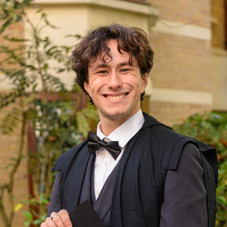
Welcome! My name is Theo, I am a PhD student at the University of Oxford. My background is in astrophysics, physical chemistry, machine learning and control.

I am broadly interested in using ML to help accelerate scientific research for the benefit of mankind. More specifically I have interests in system identification, complex systems modelling, and control. Currently, I am working on Reinforcement Learning applied to nuclear fusion. On the side, I also work on hyperoptax, a hyperparameter tuning library in pure JAX.